MLPs Are All You Need... For FLOP calculations

OK, clearly this section heading is misleading. But let me explain! So, transformer blocks are essentially made up of an attention part and a feedforward part. This feedforward block is further composed of three dense layers as below:

In maths, for a model with \(d_{\text{model}}\) embedded/model dimension and \(d_{\text{hidden}}\) hidden dimension, and an input with batch size \(N\) and sequence length \(T\), this can be written as:

\[X_{\text{out,ff}} = \sigma(X_{\text{in}} W_2 \odot X_{\text{in}} W_1) W_3\]

where \(X_{\text{in}} \in \mathbb{R}^{N\times T \times d_{\text{model}}}\), \(W_{1,2} \in \mathbb{R}^{d_{\text{model}} \times d_{\text{hidden}}}\) and \(W_{3} \in \mathbb{R}^{d_{\text{hidden}} \times d_{\text{model}}}\).

Now, lets work out the computational burden this function has for a forward pass!

There are two operations that require \(2NTd_{\text{model}}d_{\text{hidden}}\) FLOPs and memory \(d_{\text{model}}d_{\text{hidden}}\)
An element-wise multiplication which is of the order \(NTd_{\text{hidden}}\) and no memory overhead
A final operation which requires a further \(2NTd_{\text{model}}d_{\text{hidden}}\) and memory \(d_{\text{model}}d_{\text{hidden}}\)

So in total we have \(6NTd_{\text{model}}d_{\text{hidden}}\) FLOPs.

By contrast, for the Attention part, we have the following formulation:

\[A^h = \text{softmax} \left(\frac{X_{\text{in}}W^h_q \cdot {W_k^{h}}^T X_{\text{in}}^T}{\sqrt{d_h}}\right) \\ Y^h = A^h \cdot X_{\text{in}}W^h_v \\ X_{\text{out}} = Y^{h} W_{o}\]

where \(d_{\text{h}}\) is the attention head dimension, \(W_{q,k,v}^h \in \mathbb{R}^{d_{\text{model}} \times d_{\text{h}}}\), \(h\) is the attention head index which runs up to the total number of attention heads \(H\) and \(W_{o} \in \mathbb{R}^{H d_h \times d_{\text{model}}}\) .

There are three multiplications in here, each requiring \(2NTd_{\text{model}}d_{\text{h}}H\) and \(Hd_{\text{model}}d_{\text{h}}\) memory.
There is a dot product in the softmax operation which requires \(2NT^2d_{h}H\) FLOPs (where we have a squared sequence length because we’re creating the lookup table over all tokens in the sequence).
Similarly, we have another dot product between the attention matrix and the value which involves \(2NT^2d_{h}H\).
Finally, we have the last matmul operation which multiplies and reduces all the attention head outputs into our final output, which requires \(2NTd_{\text{model}}d_{\text{h}}H\) and \(Hd_{\text{model}}d_{\text{h}}\) memory.

In total, that leaves us with \(8NTd_{\text{model}}d_{\text{h}}H + 4NT^2d_{h}H\) FLOPs, where the first term is from the MLP block and the second is all down to attention.

Just to analyse this a bit more, lets investigate the relative difference between these two terms. Factoring common terms out we get:

\[4NTd_{h}H(2d_{\text{model}} + T) \simeq 8NTd_{\text{model}}d_{\text{h}}H \qquad \text{when} \quad d_{\text{model}} \gg T/2\]

where the MLPs dominate the FLOP count whenever \(d_{\text{model}}\) is higher than the context size.

Right, so now lets just put this into context. Let’s consider LLaMA 3-70B, which has \(d_{model} = 8192\) and therefore we can get a pretty good approximation to the compute costs of this model whenever our sequence length is less than ~4k tokens!

A quick note on training

The above was all done for inference, of course, for training things get slightly more complicated in terms of memory and FLOPs - especially when you start considering different checkpointing strategies for intermediate activations, different optimizer states, and other parallelisation techniques. However, we can make a simple adaptation to the FLOP calculations we did above but just considering the chain rule and backpropagation.

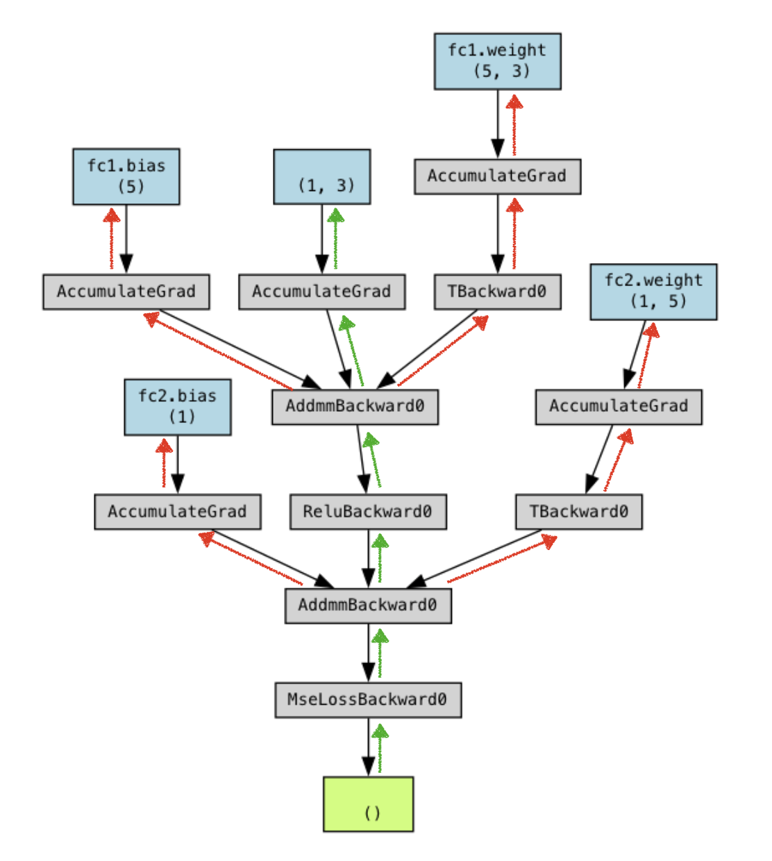
So, in training, gradients are essential for us to compute. Now imagine a set of feedforward layers stacked on top of each other, the computational graph produced from a 2-layer network looks like Figure 2.

Figure 3: Computational graph from torchviz of a 2-layer MLP with annotations to show the leaf node computations (red) and backpropgated vectors for use in previous layers through vector-Jacobian products (green). Image created by author.

The goal of backpropagation is to compute a gradient with respect to the current layer weights (this is what’s called a “leaf” in your computational graph), as well as the gradient with respect to the input of that layer.

Why do we need these? Well, the former we’re going to use in our update equation to update the weights of that layer (red path in Figure 3), and the latter we are going to pass down to the previous layer as our new vector in the vector-Jacobian-product chain (green path in Figure 3).

Don’t worry too much about the details of this here! All you need to really know is that there are 2 extra computations in the backwards pass, so you basically just want to add a factor of 3 to all the FLOP calculations we did above!