Generative Models are a class of networks which have left many of us spell-bounded in recent years. These models have propelled Artificial Intelligence (AI) into popular culture and captivated the general public by their attempts to encapsulate something inately human; creativity.

In parallel to many intricate “under-the-hood” technical advancements, the humanisation of AI has played a major role in driving the popularity of generative models. The ease of use and access to some of the most powerful AI tools the world has seen, has motivated a widespread adoption of generative models into many services and third-party applications.

Indeed, as Uncle Ben would rightly say:

with great power, comes great responsibility

and AI is no exception, with many of these new possibilities bringing with them contraversies and a new requirement for AI governance.

Anyway, we can cover AI safety and governance in another blog post. For now, in this post, I want to explain how diffusion models really work and discuss some of their incredible applications.

Problem Setup

As with all Machine Learning problems, we must start with the data! The goal of generative modelling solutions is to find some model for the data distribution such that generated outputs lie within the distribution of inputs.

Let’s just contextualise that with an example: say I asked you to imagine a car. It is highly likely that the image you choose to imagine would be similar to those you have seen in the past. In this case, your brain has a model of what a car should look like, that has been learnt from all your experience of seeing cars in the past. Therefore we can say that, the imagined output has a high probability of being close to one which is realistic to find in the wild.

To be clear, this doesn’t mean that we can imagine exactly a particular image of a car and reproduce it in our head (unless you are a slightly obsessive petrolhead…), it means we recognise the key concepts that are required for a car to be, well… a car, and we are able to compose these concepts together into something that resembles a car. Indeed, our model is not discrete and is also able to interpolate between many concepts to produce something entirely different to what we may have seen in the past. Without sounding too philisophical, this is arguably one of the pillars of human-like creativity, the compositionality of learned concepts.

Now let’s just round off this section by stating some mathematical definitions which will be useful later.

Let \(x \in \mathbb{R}^d\) be our data with dimension \(d\) which is obtained from some underlying distribution \(q_{\text{data}}(x)\). The goal of a generative model is to estimate \(p(x)\) which approximates the true data distribution \(q_{\text{data}}(x)\).

Here is an example of a model fabricating some image out of thin air!

So, how do we do this?

Setting up the training algorithm

We have data, but we don’t have any labels, so at the moment we’re in an unsupervised regime. Typically learning from unsupervised data tends to be quite hard and is also somewhat hard to control - since you are leaving the model up to its own devices.

A much easier problem would be a supervised task, so let’s try and set one of these up from the ingredients we have.

In much the same way as you would start from a blank page when asked to draw a picture, we can ask our probabilistic model to do the same. In this setting, we have the input as a randomised vector of the same dimension of \(x\) and \(x\) becomes our target! Voila!

Right, before we get confused, lets add to our math we had earlier, just so we can digest this.

Let our data be \(x^{(0)}\) and our starting point (blank page/random vector) be \(x^{(T)}\). Apologies for the cryptic notation, I promise this notation will become clearer later…

The problem we have set up is \(x^{(0)} \sim p(x^{(0)} \vert x^{(T)})\) as an approximation to \(x \sim q(x)\).

Hmm… this still seems super hard though, right? If I asked you to go from a blank page to a masterpiece in a single step, unless you were Picasso, you would quite clearly struggle. So let’s break it up, step-by-step.

Instead of going from \(x^{(T)} \rightarrow x^{(0)}\) in 1 step, lets say it takes \(T\) steps:

\[x^{(0)} \leftarrow x^{(1)} \leftarrow \dots \leftarrow x^{(t-1)} \leftarrow x^{(t)} \leftarrow \dots \leftarrow x^{(T-1)} \leftarrow x^{(T)}\]

where now we can define a much simpler regression problem at each step, which can be modelled by \(x^{(t-1)} \sim p(x^{(t-1)}\vert x^{(t)})\). With this, we can write the marginal distribution as:

\[p(x^{(0)}) = \int p(x^{(T)}) p(x^{(0)}\vert x^{(1)}) \dots p(x^{(T-1)}\vert x^{(T)}) dx^{(1)} \dots dx^{(0)} \\ = \int p(x^{(T)}) \prod_{t=1}^{T} p(x^{(t-1)}\vert x^{(t)}) dx^{(t)} \\ = \int p(x^{(0:T)}) dx^{(1:T)}\]

where the last line is a commonly used shorthand for the concatenation of variables across timesteps.

OK, so the math checks out that as long as we obey the time ordering i.e. \(x^{(T)}\) being the worst, \(x^{(0)}\) being the best and \(t=T-1,\dots 1\) being progressively better versions of \(x\).

Creating \(x^{(t)}\)

The first problem we have is that \(x^{(0)} \sim q(x^{(0)})\) is a perfect data sample, so how do we go about getting our hands on \(x^{(t)}\ \forall t \in \{1, \dots, T\}\).

This is where “noising” comes in!

The data creation process for our litter regression problems will involve noising our perfect data \(x^{(0)}\) by a small amount over \(T\) steps, until we reach \(x^{(T)}\).

We will denote the noising process as \(q(x^{(t)}\vert x^{(t-1)})\) and define it as a first order Gaussian which performs the transformation:

\[x^{(t)} = \sqrt{1-\beta_t} x^{(t-1)} + \sigma_t \epsilon_t \qquad \epsilon \sim \mathcal{N}(0,1) \\ q(x^{(t)}\vert x^{(t-1)}) = \mathcal{N}(x^{(t)}; \sqrt{1-\beta_t} x^{(t-1)}, \sigma_t^2)\]

Great! We now have our noising and denoising processing written down!

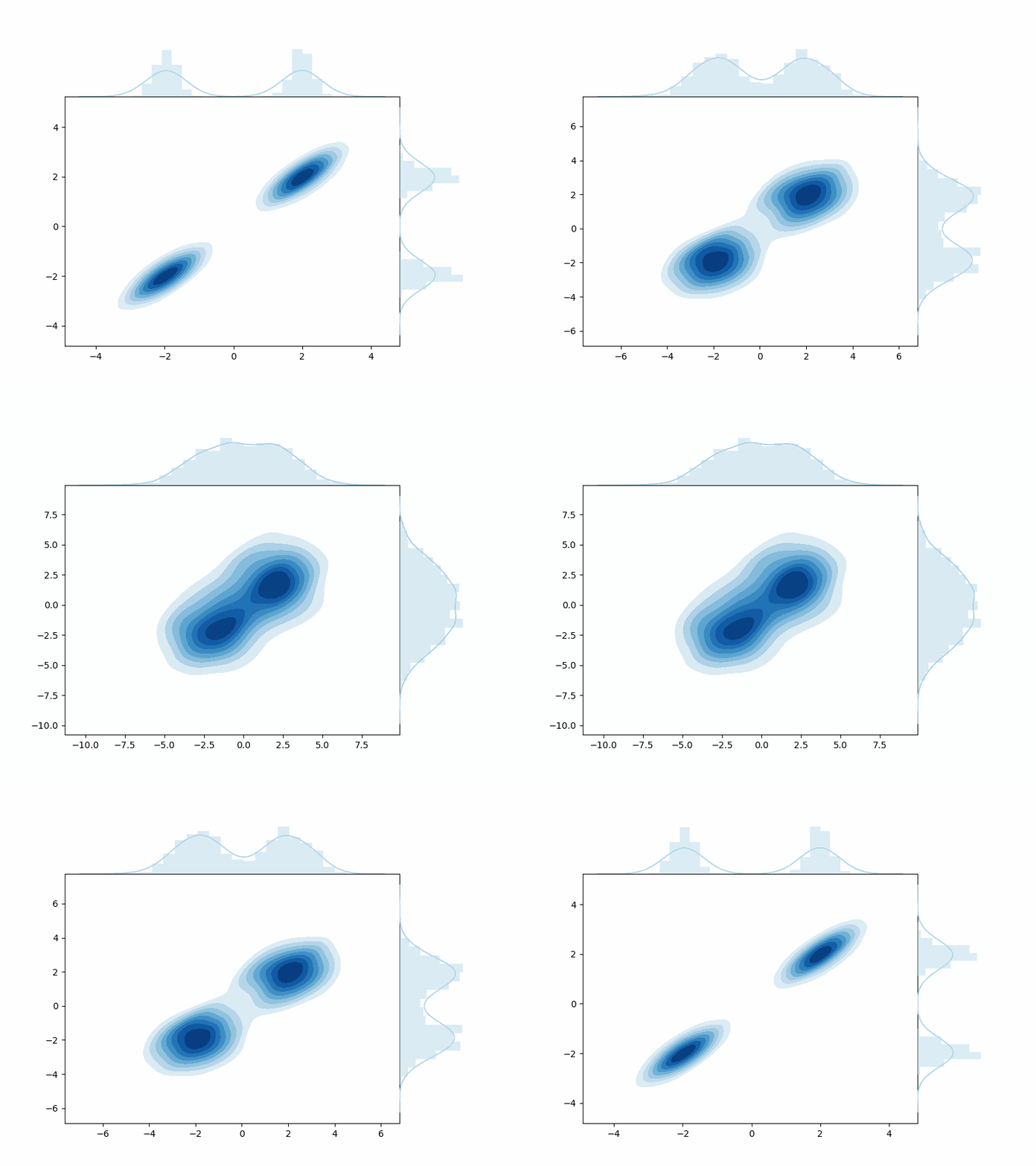
Let’s see an example of how these probabilities are related. Below is an example of how one can start with some data distribution \(q(x^{(0)})\) (with two distinct distributions) and end up with some noised Gaussian distibution - where all evidence of the original data has gone.

Aside: The View from a Frequency Perspective

I just want to pause slightly here and discuss something I find super interesting, which is; how this process looks in the frequency domain.

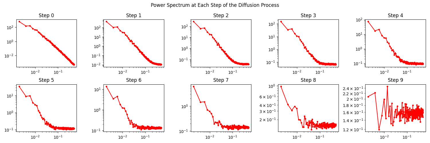
This is something that caught my eye at NeurIPS last year when I was attending a talk by Sander Dieleman (see his blog post for more inforamtion). Basically, in the frequency domain, we can think of noising as first washing out the higher frequency part of the image, before pregressively moving to dominate the lower frequency domain of the image spectra.

To unpack this more quantitatively, we can analyse the spatial frequency components of the image. When we take a Fourier transform, we produce a radial spectra which typically involves the lowest frequencies concentrated at the centre and higher frequencies at the edges. From here we can take radial slices and compute the power spectrum for that particular angle. In order to get a more global picture, we can average all of these slices and obtain whats called a Radially Averaged Power Spectral Density (RAPSD) - this is what we will play around with here. Essentially, the RASPD is a measure of the power spectrum for all spatial frequencies of an image.

Below is an animation of how this RASPD changes during the noising process:

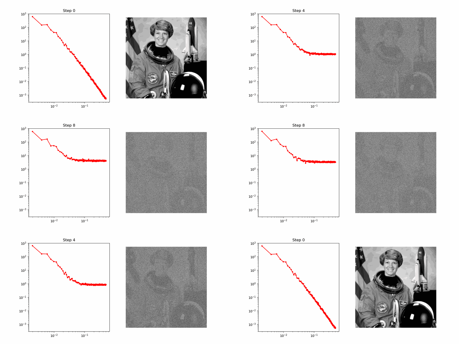
OK, so lets imagine that all these points in the RASPD are points in a sequence, in this space the denoising process (which acts in reverse to the noising process) can be viewed as an autoregressive problem, i.e. at each step, the denoising process needs to predict the next highest frequency in the sequence. Pretty cool I think!

For reference, below is the snapshots of the RASPD during the noising process!

Anyway, enough of that, now back to the main article!

How do we noise this thing?

In order to actually use this noising process, we need to first define \(\sqrt{\alpha_t} = \sqrt{1-\beta_t}\) and \(\sigma_t\). If we stop and think about what these parameters actually mean for a second, we might be able to gain some insight.

• \(\sqrt{\alpha_t} \rightarrow 0\) means that we forget all information and only have noise
• \(\sqrt{\alpha_t} = 1\) means we retain the information in \(x^{(t-1)}\)

We want \(x^{(T)}\) to contain zero information, since \(x^{(T)}\) is our blank canvas which we want to easily sample from whatever we want to generate something new.

In this sense, we would like \(\sqrt{\alpha_t} < 1\), but we want to keep small regression tasks as simple as possible - not lose too much information at each step. So we might want to have \(\sqrt{\alpha_t}\) somewhere close to 1 in practice.

As long as \(\sqrt{\alpha_t} < 1\), for \(T \rightarrow \infty\), we are guaranteed to get \(x^{(T)}\) as pure noise! - a perfect blank canvas for an ML model.

Similarly for \(\sigma_t\), this controls the amount of noise that is added at each step. Something we might want to put \(\sim 0\) for the same reasons as above.

A common choice is to set \(\sigma_t^2 = 1 - \alpha_t\), which for now we will motivate by saying that when \(\sqrt{\alpha_t} \ge 1\), \(\sigma_t^2 \ge 0\). But it is actually theoretically justified by guaranteeing that \(\mathbb{E}_{q(x^{(t)})}[x^{(t)}] = 0\) and \(\mathbb{E}_{q(x^{(t)})}[(x^{(t)})^2] = 1\).

Variance Preserving Process

Aside: \(\sigma_t^2 = 1 - \alpha_t\) ensures that \(\mathbb{E}_{q(x^{(t)})}[x^{(t)}] = 0\) and \(\mathbb{E}_{q(x^{(t)})}[(x^{(t)})^2] = 1\).

We know that the data satisfies:

\[\mathbb{E}_{q(x^{(0)})}[x^{(0)}] = 0 \quad \text{and} \quad \mathbb{E}_{q(x^{(0)})}[(x^{(0)})^2] = 1\]

because it can be normalised to do so. So let’s consider \(x^{(1)}\):

\[\mathbb{E}_{q(x^{(1)})}[x^{(1)}] = \mathbb{E}[\sqrt{\alpha_1}\ x^{(0)} + \sigma_1 \epsilon_1] = \sqrt{\alpha_1}\ \mathbb{E}[x^{(0)}] + \sigma_1 \mathbb{E}[\epsilon_1] = 0\]

because \(\epsilon_1 \sim \mathcal{N}(0, 1)\). And also:

\[\mathbb{E}_{q(x^{(1)})}[(x^{(1)})^2] = \mathbb{E}[\alpha_1 (x^{(0)})^2 + \sigma_1^2 \epsilon_1^2] = \alpha_1 \mathbb{E}[(x^{(0)})^2] + \sigma_1^2 \mathbb{E}[\epsilon_1^2] = \alpha_1 + \sigma_1^2 \\ \therefore \mathbb{E}_{q(x^{(1)})}[(x^{(1)})^2] = 1 \iff \sigma_1^2 = 1-\alpha_1\]

By recursion, we can see that this is true for all \(t\).

In this case, when the process is variance preserving, we can write down:

\[q(x^{(t)}\vert x^{(0)}) = \mathcal{N}(x^{(t)}; \prod_{i=1}^{t} \sqrt{\alpha_{i}}\ x^{(0)}, 1 - \prod_{i=1}^{t}\alpha_i)\]

which can be proved by unrolling \(q(x^{(t)}\vert x^{(t-1)})\), if you fancy doing some rather laborious maths.

OK, now we are getting somewhere. We have a problem setup, we have our chain of makeshift supervised regression problems and we know how to generate the noisey labels for each of these regression problems. Indeed, from the above, we can even generate any noisey sample at any point in this chain, directly from the input \(x^{(0)}\), as long as we have a variance preserving process!

Practically, this means that we do not need to generate all the previous \([x^{(1)}, \dots x^{(t-1)}]\) just to get \(x^{(t)}\), which will become important later when we talk about training!

Just one thing to note here before we move on to the next section is that; in order for us to generate \(x^{(0)}\) from \(x^{(T)}\), which is essentially the aim of a diffusion model, we still require \(x^{(T)}\) to be an easy sample to generate. To put this another way, when we deploy this model we will not have access to \(x^{(0)}\), we need to generate it! So our starting point \(x^{(T)}\) should ideally not have any information about \(x^{(0)}\) left inside it, it should be complete noise - which is super easy to generate independent of any other sample in the chain.

The above requirement basically tells us that we’re going to run into a balancing act between how hard we make each regression problem (how much noise we add per-step) and how many timesteps can afford to do. Anyway, more on this later!

Defining a Loss

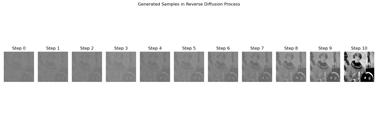
Taking a step back, we have a dataset that now consists of lots of ordered noisey samples which need to be assigined to a particular regression step in our denoising schedule (i.e., going from \(T \rightarrow\) 0).

To play aroung a bit, lets simply define a loss which concatenates all of our small regression tasks, each with their own set of parameters \(\Theta = \{\theta_t\}_{t\in [0, T-1]}\).

\[\mathcal{L}(\Theta) = \mathbb{E}_q \log\left\{p(x^{(T)}) \prod_{t=1}^{T} p_{\theta_{t-1}}(x^{(t-1)}\vert x^{(t)}) \right\} \\ =\mathbb{E}_q \left[\log p(x^{(T)})\right] + \sum_{t=1}^{T} \mathbb{E}_q \left[\log p_{\theta_{t-1}}(x^{(t-1)}\vert x^{(t)})\right]\]

where it is the second term which depends on the parameters, so an individual regression loss would be \(\mathcal{L}(\theta_{t-1}) = \mathbb{E}_q \left[\log p_{\theta_{t-1}}(x^{(t-1)}\vert x^{(t)})\right]\).

OK cool, so as we are all excellent researchers and like to think about the implications of our maths before whacking it into some code… Let’s just have a think about the complexity of the above formalism.

Let \(\theta_t \in \mathbb{R}^d\), then we will end up with a total parameter count of \(T \times d\). OK, so this means that as the number of timesteps increases, this model is going to scale linearly and as \(T \rightarrow \infty\), become intractable.

OK, you’re right, we’ll never be actually taking \(T \rightarrow \infty\) in practice. But we do need it to be pretty large to satisfy the requirements we discussed earlier, so its still a problem. One way we can try to solve this problem is weight sharing.

From now on, we will define one set of weights for all timesteps \(\theta_t \rightarrow \theta\), which reduces the total parameters to just \(d\). This is not only motivated from a computational perspective, but also by the fact that if we have defined our chain of regression tasks correctly, they are all kind of doing the same thing. So intuitively, there should be some redundancy across timesteps.

After all this, we can make a minimal adjustment to our individual loss function:

\[\mathcal{L}_{t-1}(\theta) = \mathbb{E}_q \left[\log p_{\theta}(x^{(t-1)}\vert x^{(t)})\right].\]

Right, last thing for this section, how do we add some control to this training? Let me explain…

Simply summing all the individual losses for each step in our chain is fine, but it weights each step equally in terms of its feedback to \(\theta\) - which are now shared across timesteps. However, you can imagine that there might be some steps that need to be more accurate than others in our chain.

In order to add some contol, we will introduce some weighting parameters \(w_t\) into our total loss which control how much each step contributes to updating \(\theta\):

\[\theta^{*} = \text{argmin}_{\theta} \sum_{t=1}^{T} w_{t-1} \mathcal{L}_{t-1}(\theta)\]

The Magic of Stochastic Optimization

Right now, you’re probably thinking, how much more can there be to this! But honestly, this is one of my favourite tricks that is used all over Machine Learning. Its super simple but when I first started learning about diffusion models, understanding how they leverage stochastic optimization made me think about the time axis (and also the sequence axis in transformers) in a much clearer way.

Anyway, the above update rule has a sum over \(T\) terms, all of which require varying numbers of passes through the network. This is fine but because we are sharing weights across timesteps, we can do better.

To gain an intuition, lets go back to thinking about batches of data and training a very simple neural network with parameters \(\theta\). Imagine our dataset \(\mathcal{D}\) contains \(N_\mathcal{D}\) samples. Theoretically, this gives us a solution of the form:

\[\theta^{*} = \text{argmin}_{\theta} \frac{1}{N} \sum_{n=1}^{N} w_{n} \mathcal{L}_{n}(\theta)\]

where \(w_n\) are weighting scalars for how much each sample contributes - this could be related to the quality of that datapoint for example.

This looks very similar to the equation we just wrote down for diffusion models, right? But in training a neural network we don’t need see all the \(N_\mathcal{D}\) samples, we usually get away with defining a some batches and approximating the weighted sum via an expectation over the data:

\[\frac{1}{N} \sum_{n=1}^{N} w_{n} \mathcal{L}_{n}(\theta) = \mathbb{E}_{n \sim \mathcal{U}(1,N)}[w_n \mathcal{L}_{n}(\theta)]\]

This trick is possible because the parameters are shared across mini-batches. But remember, in our diffusion setup, we are also sharing parameters across \(T\) timesteps, so we can employ exactly the same trick!

\[\theta^{*} = \text{argmin}_{\theta} \sum_{t=1}^{T} w_{t-1} \mathcal{L}_{t-1}(\theta) = \text{argmin}_{\theta} \left\{\mathbb{E}_{t \sim \mathcal{U}(1, T)} \left[w_{t-1} \mathcal{L}_{t-1}(\theta)\right]\right\}\]

Hooray, now we don’t need ALL \(T\) terms! We can just sample timesteps randomly from a uniform distribution. But remember, because we have a variance preserving process, we can get the target for the sampled timestep directly from the data \(x^{(0)}\).

The Denoising Step

Now we come to the denoising part of our pipeline… Finally!

In this part, the goal is to learn the noise which we want to remove at each step. However, because we have already defined the noising schedule with a Gaussian we can also parameterise the noise to remove similarly:

\[p(x^{(t-1)}\vert x^{(t)}; t-1, \theta) = \mathcal{N}(x^{(t-1)};\mu_{\theta}(x^{(t)}; t-1), \sigma_{\theta}^{2}(x^{(t)}; t-1))\]

This leaves us with two terms to deal with here; the mean and the variance.

For the mean, we can do this by either; (i) directly parameterising \(x^{(0)}\) at each step, or (ii) by parameterising the noise directly \(\epsilon^{(t)}\).

i. \(x^{(0)}\)-parameterisation

This method involves looking at the noising step \(q(x^{(t-1)}\vert x^{(0)}, x^{(t)})\) where from Bayes rule, we have:

\[q(x^{(t-1)}\vert x^{(0)}, x^{(t)}) \propto q(x^{(t-1)}\vert x^{(0)})q(x^{(t)}\vert x^{(t-1)}) \\ = \mathcal{N}\left( x^{(t-1)};\ \left(\prod_{t^\prime = 1}^{t-1} \sqrt{\alpha}_{t^\prime} x^{(0)} \right),\ 1 - \prod_{t^\prime = 1}^{t-1} \alpha_{t^{\prime}} \right) \times \mathcal{N}(x^{(t)};\ \sqrt{\alpha_t} x^{(t-1)}, \ 1-\alpha_t)\]

then completing the square and doing some mathematical gymnastics gives us a new distribution \(q(x^{(t-1)}\vert x^{(0)}, x^{(t)}) = \mathcal{N}(x^{(t-1)}; \mu_{t-1\vert 0,t}, \sigma_{t-1\vert 0,t}^{2})\) where:

\[\mu_{t-1\vert 0,t} = \frac{\left(\prod_{t^\prime = 1}^{t-1} \sqrt{\alpha_{t^\prime}}\right)(1-\alpha_t)}{1 - \prod_{t^\prime = 1}^{t} \alpha_{t^\prime}} x^{(0)} + \frac{\left(1 - \prod_{t^\prime = 1}^{t-1} \alpha_{t^\prime}\right)\sqrt{\alpha_t}}{1 - \prod_{t^\prime = 1}^{t} \alpha_{t^\prime}}x^{(t)} \\ \sigma_{t-1\vert 0,t}^{2} = \frac{\left(1 - \prod_{t^\prime = 1}^{t-1} \alpha_{t^\prime}\right)(1 - \alpha_t)}{1 - \prod_{t^\prime = 1}^{t} \alpha_{t^\prime}}\]

In the \(x^{(0)}\)-parameterisation, we do exactly what it says on the tin and parameterise \(x^{(0)}\):

\[\mu_{t-1\vert 0,t}^{\theta} = a^{(t)}x^{(0)}_{\theta}(x^{(t)}) + b^{(t)}x^{(t)}\]

ii. \(\epsilon\)-parameterisation

An alternative parameterisation to the above is found by instead aiming to predict the noise \(\epsilon\) at each step. Similarly to the \(x^{(0)}\)-parameterisation, our weight sharing is well-founded by the argument that each step is adding a similar amount of noise - so we can imagine some redundancy in the parameters across adjacent steps.

If we cast our minds back to earlier, we had a noising schedule which can be written as:

\[x^{(t)} = \prod_{t^\prime = 1}^{t} \sqrt{\alpha}_{t^\prime} x^{(0)} + \sqrt{1-\prod_{t^\prime = 1}^{t}\alpha_{t^\prime}}\ \epsilon^{(t)} \qquad \epsilon^{(t)} \sim \mathcal{N}(0,1) \\ x^{(t)} = c^{(t)} x^{(0)} + d^{(t)} \epsilon^{(t)}\]

So if we take the conditional mean that we got from our \(x^{(0)}\)-parameterisation, we can easily substitue the above into this and write down a new expression of the form:

\[\mu_{t-1\vert 0,t}^{\theta} = \left(\frac{a^{(t)}}{c^{(t)}} + b^{(t)}\right)x^{(t)} - \frac{a^{(t)}d^{(t)}}{c^{(t)}}\epsilon^{(t)}_{\theta}(x^{(t)})\]

So given the input and the timestep, our parameterisation now predicts the noise that needs to be taken away from \(x^{(t)}\) in order to give \(x^{(t-1)}\).

OK, so hopefully its pretty easy to see how these two parameterisations are related to each other. In fact, you might be asking, “what is the difference?” or “why would we want to do this?” - these would be valid questions!

To answer these a bit more in depth, we can consider how each one is actually performing the denoising step and at the same time, learn about some related work!

Denoising Autoencoders (DAE)

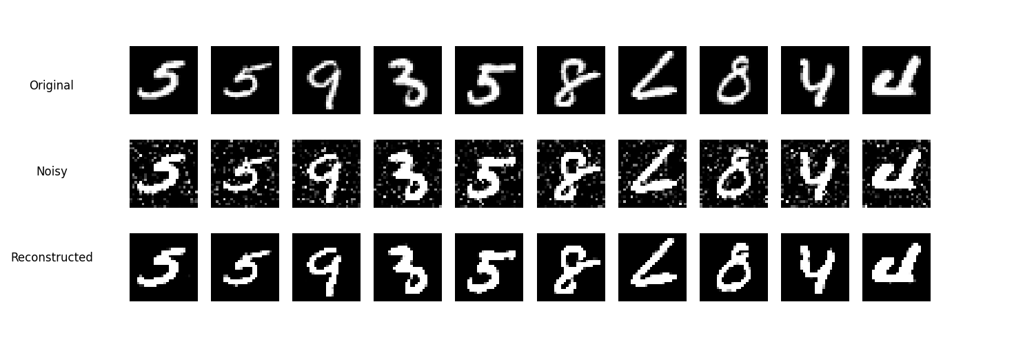
As discussed above, in the \(x^{(0)}\)-parameterisation, the goal is to predict the clean data \(x^{(0)}\) from a noisy version \(x^{(t)}\). The DAE is trained to map the noisy input \(x^{(t)}\) to the clean output \(x^{(0)}\). This process can be formulated as: \(x_{\theta}^{(0)} = f_{\theta}(x^{(t)})\)

where \(f_\theta\) is the neural network which parameterises \(x_\theta^{(0)}\), \(x^{(t)}\) is the noisy input at time step \(t\), and \(x^{(0)}\) is the predicted clean data.

The training objective for the DAE in this context is to minimize the mean squared error (MSE) between the predicted clean data \(x_{\theta}^{(0)}\) and the actual clean data \(x^{(0)}\):

\[\mathcal{L}_{DAE} = \mathbb{E}_{x_0, t, \epsilon} \left[ | x^{(0)} - f_\theta(x^{(0)}+\epsilon) |^2 \right]\]

Here, \(\epsilon\) represents the noise added to the clean data \(x^{(0)}\) to obtain \(x^{(t)}\). Taking a look at our objective for the \(x^{(0)}\)-parameterisation, we are aiming to achieve something which is \(\propto x^{(0)} - x^{(0)}_{\theta}(x^{t}, t-1)\).

Seeing it this way, we can see the resemblance of the denoising autoencoder to this specific parameterisation of a diffusion model.

Denoising Score Matching (DSM)

Denoising score matching (DSM) is a technique used to estimate a score function. The score function is defined as the gradient of the log probability density function of the data. OK, slow down, what does that mean?

Well, remember that \(q(x^{(t-1)}\vert x^{(0)}, x^{(t)})\) is our noising process. The score is the change in this noising process across the noising schedule, which changes with \(x\). In the context of diffusion models, DSM is therefore closely related to the \(\epsilon\)-parameterisation, which essentially parameterises the change between steps in the noising process.

In the \(\epsilon\)-parameterisation, the objective is to predict the noise added to the clean data \(x^{(0)}\) to obtain the noisy data \(x^{(t)}\). A neural network \(g_\theta\) is trained to map the noisy input \(x^{(t)}\) to the noise $$\epsilon:

\[\epsilon_{\theta} = g_{\theta}(x^{(t)})\]

As with our DAE discussion, lets have a look at a simple DSM training objective:

\[\mathcal{L}_{DSM} = \mathbb{E}_{x_0, t, \epsilon} \left[ | \epsilon - g_\theta(x^{(t)}) |^2 \right]\]

By minimizing this loss, the neural network learns to accurately predict the noise, which is essential for the \(\epsilon\)-parameterisation of diffusion models.

Now we mentioned a score function, which is written as \(\nabla_{x^{(t)}}\log p(x^{(t)})\) indirectly. Since the noise \(\epsilon\) is related to the score function through the gradient of the log probability density, predicting \(\epsilon\) effectively helps in estimating the score function.

Anyway, score matching is an interesting topic which I’m not going to dwell too much on here but essentially it shares many concepts with denoising diffusion models - where the \(\epsilon\)-parameterisation is basically practical implementation of score matching.

Defining a Loss Function

OK, we’ve been around the block a bit and discussed some technical stuff, but just to wrap up this post, I’m going to drop a loss function here which was introduced by Ho, et. al., (2020) in the seminal paper on denoising diffusion models:

\[\mathcal{L}(\theta) = -\frac{T}{2}\mathbb{E}_{t}\left[\left(\epsilon^{(t)} - \epsilon^{(t)}_{\theta}(\sqrt{\alpha_t} x^{(0)} + \sqrt{1-\bar{\alpha}_t} \epsilon^{(t)}, t-1)\right)^2\right]\]

where \(\bar{\alpha}_{t} = \prod_{t^\prime=1}^{t}alpha_{t^\prime}\). Hopefully, you are able to see that this loss function follows quite nicely from some of the discussions we have had in earlier sections.

OK, great! Thanks for reading this post, if you have made it this far! Although technical, I hope it has given you a bit more of an intuitive explanation behind some of the main mathematical concepts of diffusion models.

References

There are loads of references that I could state here. These are a few which inspired this post and/or that I find useful!

• J. Ho, et. al., Denoising Diffusion Probabilistic Models, (2020)
• L. Weng, What are Diffusion Models?, (2021)
• S. Dieleman, Diffusion is Spectral Autoregression, (2024)
• R. Turner, Denoising Diffusion Probabilistic Models in Six Simple Steps, (2024)
• I. Strümke, H. Langseth, Lecture Notes in Probabilistic Diffusion Models, (2023)