Convexity Explained

What is convexity?

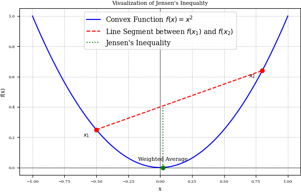
A function is convex if the line segment between two points lies above the function.

In the above figure, we see an illustrative example of the definition above. Here, we can see that if the intersection of the line forms an enclosed area which is uninterrupted above the curve, the function can be considered convex.

We can also see that if the opposite is true i.e. the enclosed area is below the curve, the function is concave!

Indeed, a convex function \(f(x)\) can be reflected into a concave function \(-f(x)\).

Mathematically, convexity is best described by Jensen’s inequality,

\(f(E[X]) \le E[f(X)]\) for a convex function \(f\) and a random vector \(X\) that is within the domain of \(f\). Now, I find it hard to conceptualise inequalities at face value, so let’s chat about it a bit…

Jensen’s inequality essentially states that the expected value of a convex transformation of a random variable (i.e. \(E[f(X)]\)) is more than or equal to the value of the convex function evaluated at the mean od the random variable (i.e. \(f(E[X])\)) - or the gap between these two is never negative.

OK, I’ll be honest, when I wrote that, it only half made sense to me… I’m a physicist by background and so I love drawings and building intuitions visually, so let’s do that!

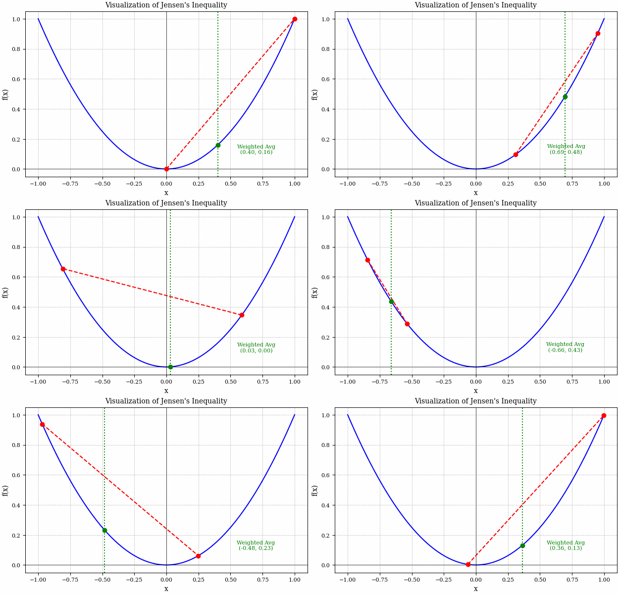
Consider the figure above, here it is a lot easier to see what Jensen’s inequality is really saying. Basically the LHS of Jensen’s inequality is represented by the green dotted line - this is taking the average of the two red \(x\) points and then evaluating the function at this point (i.e. \(f(E[X])\)). Whereas, the intersection of the red dashed line and the green dotted line is what the RHS of Jensen’s inequality is describing - evaluating the function before taking the expectation (i.e. \(E[f(X)]\)).

We can see that over the entire range of this function, the green dot never crosses the red line and so the intersection of the green dotted and red dashed lines is always above the blue solid curve.

OK, hopefully that was a nice and easy to follow explanation for you! And if it wasn’t, at least you got to distract yourself with a cool animation! Anyway, let’s get back to convexity…

OK, so as well as Jensen’s inequality, for a twice differentiable function which is convex, we have two rather nice conditions:

The first of these conditions tells us that curvature must be positive everywhere. The second condition ensures that the line between two points \(x\) and \(y\) lies above the function within that interval (illustrated earlier).

Following on from this, the first condition ensures that a convex function must curve upwards (or not at all). Therefore, if we find a minima x, any movement away from this point will result in an increase in the function value.

Together, these conditions are enough to guarantee that any minima found in a convex function must be a global minima (although this doesn’t necessarily need to be unique). This is extremely useful for techniques such as stochastic Gradient Descent since if we find a local minima (something which Gradient Descent generally tends to find), we can be certain that this in fact the global minima - the best possible solution.

The Strong, the Strict and the Standard

As always with math, we don’t just have one type of something, we have some vague terms that sound cool to describe some more features.

Convex functions are no exception and can be further categorised with three properties:

• Convex
• Strictly Convex
• Strongly Convex

Now, the further you move down that list, the stronger these properties become (hence the “strongly” term). This just means that the subset of convex functions that have these properties becomes smaller due to stronger constraints.

So far in this post, we have been talking about convexity in its most general form, where \(f^{''}(x) >= 0\). This is the condition for ‘convex’ functions.

Strictly convex functions are those which satisfy \(f^{''}(x) > 0\), i.e. the curvature can never be 0.

Stongly convex functions are those which satisfy \(f^{''}(x) >= m > 0\), where the curvature is non-vanishing and stays bounded below by some positive value \(m\).

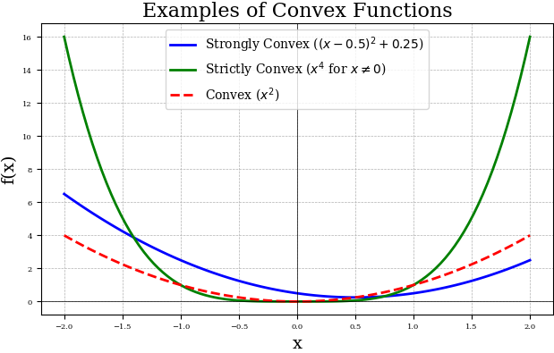
In the above plot, we can see the differences between these types of convexities visually. If you take the definitions in the legend and differentiate these twice then it is easy to prove to yourself that each of these are convex, strictly convex or strongly convex.

OK cool, well done for reading another one of my posts! I’m trying to keep these as short and sweet as possible and just give the “need-to-know” understanding for these concepts. Let me know how I did!